
#8. Pytorch 실습
2022. 11. 1. 15:41
Update Log
| 22.10.05 First Update
이번 포스팅에서...
그동안 배워왔던 개념들을
colab을 통해서 pythorch 를 이용한 실습을 할
예정이다.
선형회귀 (Linear Regression)
import torch
import numpy as np
inputs = np.array([[2],[4],[6],[8]],
dtype='float32')
#input 값
targets = np.array([3,4,5,6],
dtype='float32')
#output 값inputs = torch.from_numpy(inputs)
targets = torch.from_numpy(targets)
#텐서로 바꿔서 활용하는 부분from torch.utils.data import TensorDataset, DataLoader
dataset = TensorDataset(inputs, targets)
loader = DataLoader(dataset, batch_size=4)
# 이 부분은 굳이 사용하지 않아도 되는 부분w = torch.randn(1,1,requires_grad= True)
b = torch.randn(1, requires_grad= True)
# 초기화 및 정의def model(X):
return X @ w.t()+bdef mse_loss(predictions, targets):
difference = predictions - targets
return torch.sum (difference * difference)/ difference.numel()for x,y in dataset:
preds = model(x)
print(f'Prediction: {preds.item():.2f} / Actual target: {y.item():.2f} / loss: {mse_loss(preds, y):.2f}')출력값
Prediction: 2.33 / Actual target: 3.00 / loss: 0.45
Prediction: 3.11 / Actual target: 4.00 / loss: 0.78
Prediction: 3.90 / Actual target: 5.00 / loss: 1.21
Prediction: 4.69 / Actual target: 6.00 / loss: 1.73
#학습하는 부분
epochs = 10000 #학습을 10000번 반복하겠다.
for i in range(epochs):
for x,y in loader:
# Generate Prediction
preds = model (x)
# Get the loss and perform backpropagation
loss = mse_loss(preds[:,0],y)
loss.backward()
# Let's update the weights
with torch.no_grad():
w -= w.grad*1e-3
#running rate 가 1/1000 이다.
b -= b.grad * 1e-3
# Set the gradients to zero
w.grad.zero_()
b.grad.zero_()
#print(f"Epoch {i}/{epochs}: Loss: {loss}")for x,y in dataset:
preds = model(x)
print(f'Prediction: {preds.item():.2f} / Actual target: {y.item():.2f} / loss: {mse_loss(preds, y):.2f}')Prediction: 2.99 / Actual target: 3.00 / loss: 0.00
Prediction: 3.99 / Actual target: 4.00 / loss: 0.00
Prediction: 5.00 / Actual target: 5.00 / loss: 0.00
Prediction: 6.01 / Actual target: 6.00 / loss: 0.00import matplotlib.pyplot as plt
x_tmp = np.arange(0,11,1)
y_tmp = w.detach().numpy()*x_tmp+b.detach().numpy()
plt.plot(inputs,targets,'x')
plt.plot(x_tmp,y_tmp[0])
plt.xlabel('x')
plt.ylabel('y')
plt.show()
#파란색 점은 우리가 가지고 있는 데이터, 노란색 선은 우리가 구했던 모델이라고 생각하면 된다
퍼셉트론
import torch
import numpy as np
inputs = np.array([[0,0],[0,1],[1,0],[1,1]], dtype='float32')
targets = np.array([0,1,1,1], dtype='float32')
#targets = np.array([0,0,0,1], dtype='float32')
#targets = np.array([0,1,1,0], dtype='float32')inputs = torch.from_numpy(inputs)
targets = torch.from_numpy(targets)from torch.utils.data import TensorDataset, DataLoader
dataset = TensorDataset(inputs, targets)
loader = DataLoader(dataset, batch_size=4)w = torch.randn(1,2,requires_grad=True) #입력층 2차원
w0 = torch.randn(1,requires_grad=True) #바이어스 텀def model(X):
return torch.sigmoid(X @ w.t()+w0) #원래 퍼셉트론에서는 계단함수인데 미분을 위해서 여기에서는 시그모이드 사용criterion = torch.nn.BCELoss() #binaryclassification의 손실함수 정의for x,y in dataset:
preds = model(x)
print(f'Prediction: {preds.item():.2f} / Actual target: {y.item():.2f}')Prediction: 0.45 / Actual target: 0.00
Prediction: 0.11 / Actual target: 1.00
Prediction: 0.39 / Actual target: 1.00
Prediction: 0.09 / Actual target: 1.0epochs = 1000
for i in range(epochs):
for x,y in loader:
# Generate Prediction
preds = model(x)
# Get the loss and perform backpropagation
loss = criterion(preds[:,0],y)
loss.backward()
# Let's update the weights
with torch.no_grad():
w -= w.grad
w0 -= w0.grad
# Set the gradients to zero
w.grad.zero_()
w0.grad.zero_()
# print(f"Epoch {i}/{epochs}: Loss: {loss}")for x,y in dataset:
preds = model(x);
print(f'Prediction: {preds.item():.2f} / Actual target: {y.item():.2f}')Prediction: 0.02 / Actual target: 0.00
Prediction: 0.99 / Actual target: 1.00
Prediction: 0.99 / Actual target: 1.00
Prediction: 1.00 / Actual target: 1.00import matplotlib.pyplot as plt
x1_tmp = np.arange(-0.2,1.3,0.1)
w_tmp = w.detach().numpy()
x2_tmp = (-w_tmp[0,0]*x1_tmp-w0.detach().numpy())/w_tmp[0,1]
fig = plt.figure()
ax = fig.add_subplot(111)
for i in range(len(inputs)):
if targets[i] == 1:
plt.plot(inputs[i,0],inputs[i,1],'bx')
else:
plt.plot(inputs[i,0],inputs[i,1],'rd')
plt.plot(x1_tmp,x2_tmp)
plt.xlim([-0.2,1.2])
plt.ylim([-0.2,1.2])
plt.xlabel('x1')
plt.ylabel('x2')
ax.set_aspect('equal')
plt.show()
퍼셉트론 (Library Version)
import torch
import numpy as np
inputs = np.array([[0,0],[0,1],[1,0],[1,1]], dtype='float32')
#targets = np.array([0,1,1,1], dtype='float32')
#targets = np.array([0,0,0,1], dtype='float32') #and
targets = np.array([0,1,1,0], dtype='float32') #XORinputs = torch.from_numpy(inputs)
targets = torch.from_numpy(targets)from torch.utils.data import TensorDataset, DataLoader
dataset = TensorDataset(inputs, targets)
loader = DataLoader(dataset, batch_size=4)linear = torch.nn.Linear(2,1,bias = True)
sigmoid = torch.nn.Sigmoid()model = torch.nn.Sequential(linear, sigmoid) #라이브러리로 퍼셉트론을 간단하게 설명하는 부분이다.criterion = torch.nn.BCELoss()
optimizer = torch.optim.SGD(model.parameters(), lr=1)for x,y in dataset:
preds = model(x)
print(f'Prediction: {preds.item():.2f} / Actual target: {y.item():.2f}')Prediction: 0.63 / Actual target: 0.00
Prediction: 0.66 / Actual target: 1.00
Prediction: 0.47 / Actual target: 1.00
Prediction: 0.50 / Actual target: 0.00epochs = 1000
for i in range(epochs):
for x,y in loader:
# Generate Prediction
preds = model(x)
# Get the loss and perform backpropagation
loss = criterion(preds[:,0],y)
loss.backward()
# Let's update the weights
optimizer.step() #step이라는 함수를 적용해서 그래디언트를 구해서 w,와 w0를 옮겨라는 것을 이야기해줌
# print(f"Epoch {i}/{epochs}: Loss: {loss}")for x,y in dataset:
preds = model(x)
print(f'Prediction: {preds.item():.2f} / Actual target: {y.item():.2f}')Prediction: 0.43 / Actual target: 0.00
Prediction: 0.41 / Actual target: 1.00
Prediction: 0.58 / Actual target: 1.00
Prediction: 0.56 / Actual target: 0.00import matplotlib.pyplot as plt
x1_tmp = np.arange(-0.2,1.3,0.1)
w_tmp = []
for param in model.parameters():
w_tmp.append(param.data)
x2_tmp = (-w_tmp[0][0,0].numpy()*x1_tmp-w_tmp[1].numpy())/w_tmp[0][0,1].numpy()
fig = plt.figure()
ax = fig.add_subplot(111)
for i in range(len(inputs)):
if targets[i] == 1:
plt.plot(inputs[i,0],inputs[i,1],'bx')
else:
plt.plot(inputs[i,0],inputs[i,1],'rd')
plt.plot(x1_tmp,x2_tmp)
plt.xlim([-0.2,1.2])
plt.ylim([-0.2,1.2])
plt.xlabel('x1')
plt.ylabel('x2')
ax.set_aspect('equal')
plt.show()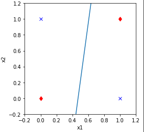
'STUDY > 인공지능' 카테고리의 다른 글
| #10. CNN (0) | 2022.11.28 |
|---|---|
| #9. 딥러닝 주요 최적화 방법 (0) | 2022.11.01 |
| #7. 딥러닝과 깊은 퍼셉트론 (0) | 2022.11.01 |
| #6. 다층 퍼셉트론 및 딥러닝 기초 (0) | 2022.11.01 |
| #5. 최적화 이론 (1) | 2022.11.01 |